Physics-Based 3D Ball Trajectory Reconstruction from Monocular Soccer Video: A Multi-Model Benchmark

Łukasz Grad^1,2,*    Krzysztof M. Czajkowski^2,*    Aliaksandr Varashylau^2,*

¹University of Warsaw, Poland    ²ReSpo.Vision, Poland ^*Equal contribution · 📧 l.grad@mimuw.edu.pl

🔍 Overview

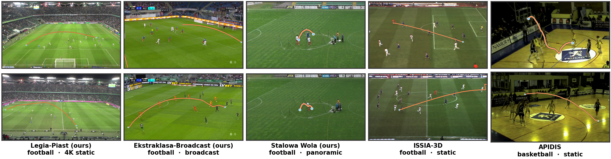
TL;DR. We benchmark seven physics-based arc models — from gravity-only parabolas to MuJoCo simulations with drag, spin, and fluid forces — for reconstructing 3D soccer-ball trajectories from monocular video. The pipeline segments each trajectory at contact events and fits every segment by optimizing a forward-simulated flight model against a reprojection-based objective. Across five datasets (~6,000 trajectory segments), the monocular and oracle-3D protocols yield reversed model rankings: a fitted-gravity model wins under monocular reconstruction while a spin-decomposition model leads when fitted to 3D ground truth — suggesting that observation noise and single-view geometric ambiguity, not model expressiveness, are the primary limiting factors. We publicly release two new soccer datasets with triangulated 3D ground truth, plus segment-level annotations for APIDIS and ISSIA-3D.

Installation

uv sync

Data

See DATA.md for datasets, download link, per-clip layout, conventions, and file-by-file schemas.

Running Experiments

All scripts use Hydra for configuration. Always run via uv run.

See conf/base.yaml for global parameters and conf/trajectory/ for estimator-specific configs.

Pipeline order: raw detections → preprocess_trajectory → estimate_trajectory → evaluate_trajectory / visualize_trajectory. The GDrive dataset ships preprocessing output and per-model predictions, so the typical starting point is evaluate_trajectory or visualize_trajectory.

Preprocessing (optional)

The GDrive dataset already ships the preprocessing output dev/df_merged_ball_player.csv for every view-sequence, so most users can skip this step. Run it only if you want to regenerate from raw detections.

uv run python preprocess_trajectory.py \
    root=data/ISSIA/camera01/half_1 \
    version=test

Requires player detections (detection/detection.feather) under <root>/detection/.

Trajectory Estimation

uv run python estimate_trajectory.py \
    trajectory=basic_angular_velocity \
    root=data/stalowa_wola_5/pano/clip \
    version=basic_angular

Writes <root>/track/ball_3d.<version>.csv. The <root> path depends on the dataset (see the Data structure examples).

Visualization

Render a model's 3D trajectory overlaid on the source video. Requires input.mkv in <root> (LP and SW pano only).

uv run python visualize_trajectory.py \
    root=data/stalowa_wola_5/pano/clip \
    version=basic_angular

Add visualisation.show_ground_truth=true to also overlay the ground-truth trajectory:

uv run python visualize_trajectory.py \
    root=data/stalowa_wola_5/pano/clip \
    version=basic_angular \
    visualisation.show_ground_truth=true

Evaluation

Compute per-clip metrics (mAP at multiple distance thresholds, 3D errors broken down by full / arc / straight, coverage, etc.) for a model's predictions:

uv run python evaluate_trajectory.py \
    root=data/stalowa_wola_5/pano/clip \
    trajectory=basic_angular_velocity version=basic_angular

Writes <root>/eval/gt_metrics-<version>.json, <root>/eval/errors-<version>.csv, and diagnostic plots. The JSON contains every metric reported in paper Tables 3 and 5.

Available Trajectory Estimators

The seven physics models from the paper (Table 1):

Config	Paper name	Description
basic_kinetic_estimator_parabola	basic parabola	Pure ballistic motion under gravity; no drag, no spin
basic_kinetic_estimator	basic kinetic	Gravity + quadratic drag (k3)
basic_kinetic_fitg	basic fitg	Drag (k3) + fitted gravitational constant g (proxy for unmodelled effects)
basic_angular_velocity	basic angular	Drag + Magnus force decomposed into lift (kl, topspin/backspin) and sidespin (ks)
mujoco_kinetic_estimator	MuJoCo kinetic	MuJoCo simulation with fixed inertia-based fluid drag (no fitted aero params)
mujoco_angular_velocity	MuJoCo angular	MuJoCo with fitted initial angular velocity ω₀
mujoco_ellipsoid_angular_velocity	MuJoCo ellipsoid	MuJoCo ellipsoid fluid model: blunt drag, angular drag, Magnus, with fitted ω₀

For the arc-loss ablation (paper Table 6, supplement §8.1), six additional configs match basic_parabola and basic_fitg but zero out individual loss-objective terms (L_end, L_z, or both):

• basic_kinetic_estimator_parabola_{no_end,no_z,traj_only}.yaml
• basic_kinetic_fitg_{no_end,no_z,traj_only}.yaml

Common Overrides

# Parallel jobs
n_jobs=8

# Frame stepping
step_frame=1

# Time range
start_sec=0 end_sec=-1

# Use ground truth pivot points
use_gt_pivots=true

Reproducing paper tables

Three shell scripts run evaluation across a dataset and macro-average the per-view results into a CSV matching the paper layout. Each assumes ball_3d.<version>.csv predictions already exist under each ROOT.

Script	Reproduces	Default ROOTS
./eval_table3.sh	Table 3 (mAPbal, mAParc per model)	LP-static (cameras 01–05 × 2 halves)
./eval_table5.sh	Table 5 (Full / Str / Arc mean 3D error, m, for the two best models)	LP-static (cameras 01–05 × 2 halves)
./eval_table6.sh	Table 6 (arc-loss ablation, mAParc and vertical error, 8 model × objective variants)	LP-static (cameras 01–05 × 2 halves)

What each script does:

1. Calls evaluate_trajectory.py for every (root, model) pair to produce per-half eval/gt_metrics-<version>.json.
2. Macro-averages the relevant fields across roots.
3. Writes logs/table<N>.csv.

Edit the ROOTS=(...) array at the top of a script to switch dataset columns. eval_table3.sh and eval_table5.sh ship with a commented-out LP-broadcast block alongside the active LP-static one; eval_table6.sh is LP-static only (per paper §8.1).

Env vars:

OUTPUT_CSV=logs/table3-lp-static.csv  # override output path
SKIP_EXISTING=1                       # reuse existing eval/gt_metrics-<ver>.json

✏️ Citation

If you find this work useful, please cite our paper:

@InProceedings{Grad_2026_CVPR,
    author    = {Grad, {\L}ukasz and Czajkowski, Krzysztof M. and Varashylau, Aliaksandr},
    title     = {Physics-Based 3D Ball Trajectory Reconstruction from Monocular Soccer Video: A Multi-Model Benchmark},
    booktitle = {Proceedings of the IEEE/CVF Conference on Computer Vision and Pattern Recognition (CVPR) Workshops},
    month     = {June},
    year      = {2026},
    pages     = {9940-9948}
}

📄 License

This project is licensed under the CC-BY-NC-SA-4.0 license.